Capacitor Charge and Discharge

A LevelAQA

Capacitor Charge and Discharge Revision

Capacitor Charge and Discharge

For this unit it is important to be able to read and interpret the shapes of charging and discharging graphs for capacitors. For each we need to know the graphs of current, potential difference and charge against time.

Charging Graphs

As previously mentioned, work is done on the electrons in the circuit to overcome the electrostatic forces present in a capacitor. At the positive plate, electrons are attracted back towards the plate but the potential difference of the supply overcomes this force. Similarly at the negative plate, electrons from the circuit have to overcome the repulsive forces between the like charges.

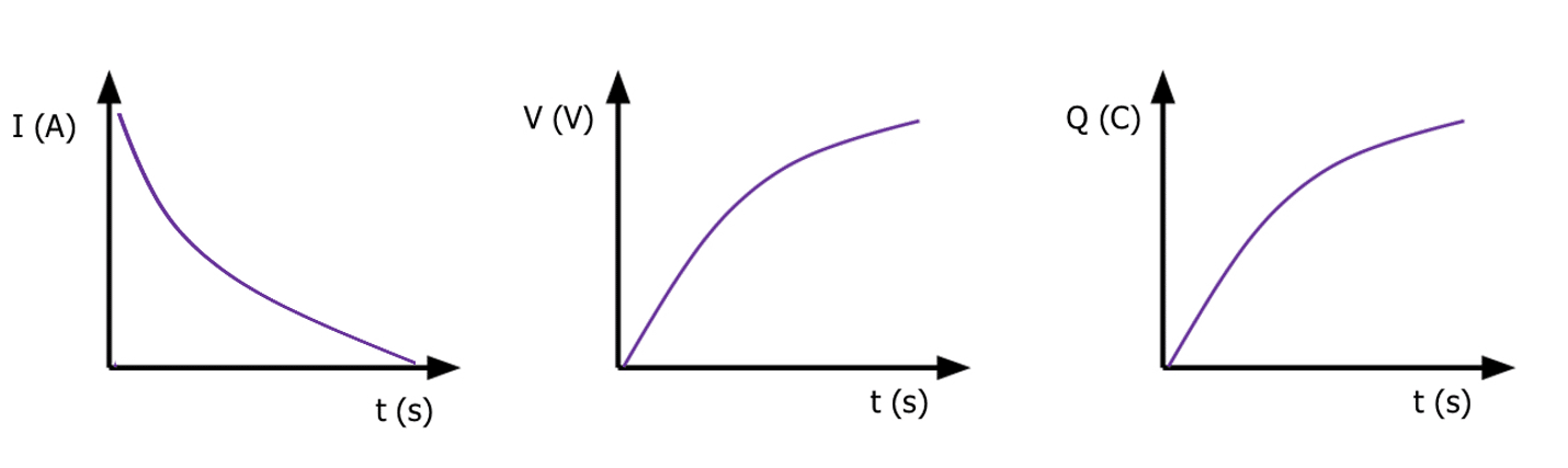
As seen in the current-time graph, as the capacitor charges, the current decreases exponentially until it reaches zero. This is due to the forces acting within the capacitor increasing over time until they prevent electron flow.

The potential difference needs to increase over time exponentially as does charge. This is because of the build-up of electrons on the negative plate and the removal of electrons on the positive plate over time. The potential difference increases until it reaches an equal potential difference as the power supply. The maximum charge is determined by the rating of the capacitor.

Discharging graphs

When a capacitor discharges, it always discharges through a resistor when disconnected from the power supply (or the power supply is switched off).

As soon as the power supply is switched off and the capacitor is connected to the resistor, it rapidly discharges causing the electrons on the negative plate to return to the positive plate until the p.d reaches zero.

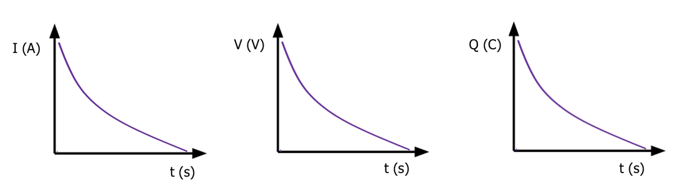
All three graphs for discharging are identical exponential decay curves.

As the electrons stop flowing from the negative plate to the positive plate, the current, potential difference and charge all return to zero. The capacitor is ready to be charged again by connecting back to the power supply.

To increase the rate of discharge, the resistance of the circuit should be reduced. This would be represented by a steeper gradient on the decay curve.

The Time Constant

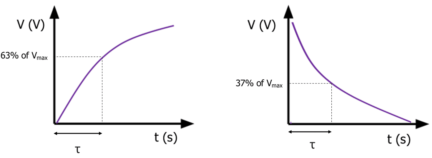
The time constant of a discharging capacitor is the time taken for the current, charge or potential difference to decrease to $37 \%$ of the original amount. It can also be calculated for a charging capacitor to reach $63 \%$ of its maximum charge or potential difference.

The time constant $\left(\tau\right)$ is proportional to the resistance and the capacitance of the capacitor. This can be represented in the equation:

$\tau = RC$

$\tau$ is the time constant in seconds $\left(\text{s}\right)$
$R$ is the resistance of the resistor connected to the capacitor in ohms $\Omega$
$C$ is the capacitance in the capacitor $\left(\text{F}\right)$

Example: Calculate the time constant for a $10 \: \text{nF}$ capacitor discharging through a $500 \: \text{k} \Omega$ resistor.

[1 mark]

$\tau = RC$

$\tau = 500 \times 10^3 \times 10 \times 10^{-9} = 5 \times 10^{-3} \: \text{s} \: \text{or} \: 5 \: \text{ms}$

Alternatively, the time constant can be found using a voltage-time graph for a capacitor by reading the time from the graph when the voltage of a charging capacitor reaches $63 \: \%$ or the voltage of a discharging capacitor reaches $37 \: \%$ .

As both charging and discharging graphs are exponential graphs, the $63 \: %$ (or $0.63$ ) is the exponential function $\left(e\right)$ whilst the $37 \: \%$ for a discharging capacitor is equal to $\dfrac{1}{e}$ .

It is also useful to note that the time to charge/discharge to half the amount of charge is given by:

$T_{1/2} = 0.69 RC$

Charging and Discharging equations

Using the time constant $\left(\tau\right)$ , we can calculate the amount of current, charge or p.d left after an amount of time discharging. The equations we use are:

$I = I_0 e^{-t/RC}$

$I$ is the current in amps $\left(\text{A}\right)$ , $I_0$ is the initial current, $t$ is the time and $RC$ is the time constant.

$V = V_0 e^{-t/RC}$

$V$ is the voltage in volts $\left(\text{V}\right)$ , $V_0$ is the initial p.d, $t$ is the time and $RC$ is the time constant.

$Q = Q_0 e^{-t/RC}$

$Q$ is the charge in coulombs $\left(\text{C}\right)$ , $Q_0$ is the initial charge, $t$ is the time and $RC$ is the time constant.

For a capacitor charging, we can use the following equation:

$Q = Q_0 \left(1-e^{-t/RC}\right)$

where the elements of the equation have the same meaning, however $Q_0$ is the maximum charge of the capacitor.

Example: Calculate the current after $0.2$ seconds for a $0.8 \: \text{mF}$ capacitor discharges from an initial current of $0.5 \: \text{A}$ through a $500 \: \Omega$ resistor.

[3 mark]

$I = I_0 e^{-t/RC}$

$\text{Time Constant} \left(RC\right) = 500 \times 0.8 \times 10^{-3} = 0.4 \: \text{s}$

$I = 0.5 \times e^{-0.2/0.4}$

$I = 0.3 \: \text{A}$

Required Practical 9

Investigating Charging and Discharging Capacitors.

This experiment will involve charging and discharging a capacitor, and using the data recorded to calculate the capacitance of the capacitor. It’s important to note that a large resistance resistor (such as a $10 \: \text{kΩ}$ resistor) is used to allow the discharge to be slow enough to measure readings at suitable time intervals.

We will measure the time taken for a capacitor to discharge in this method. A similar experiment could be conducted where you measure the time taken for the capacitor to charge instead.

Doing the experiment:

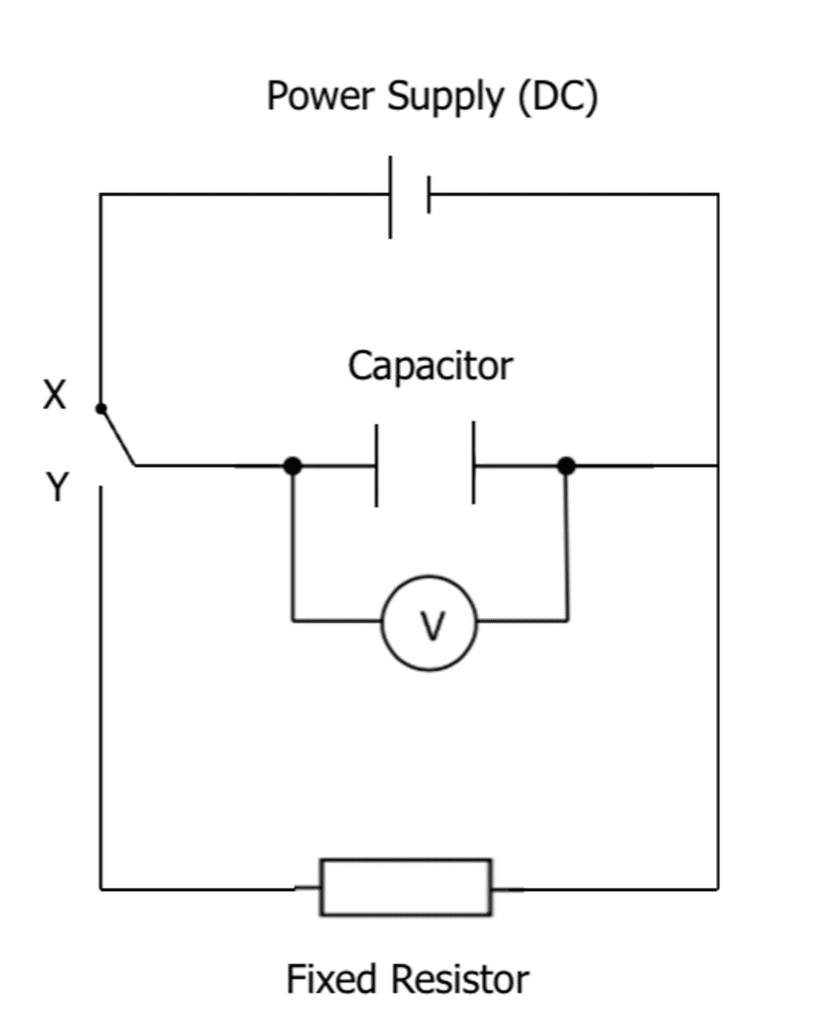
Set up the circuit as shown, however ensure the switch is open (not connected to X or Y). You will also need a stopwatch for this experiment.
The capacitor at this stage should be fully discharged as no current has yet passed through the capacitor.
Set the power supply to $10 \: \text{V}$ .
Move the switch to position X, which will begin charging the capacitor. You can tell when the capacitor is fully charged when the voltmeter reading reads $10 \: \text{V}$ .
Once fully charged, the switch should be moved to position Y and the capacitor will begin discharging.
Record the voltage on the voltmeter every $10$ seconds until the capacitor has fully discharged $\left(0 \: \text{V}\right)$ .

Analysing the results:

We know from earlier in this page that the equation for a capacitor discharging in terms of voltage is:

$V = V_0 e^{-t/RC}$

If we want to calculate the capacitance $C$ using our results in the experiment, we need to rearrange this equation.

First if we take the natural log of both sides:

$\text{ln}\left(\dfrac{V}{V_0}\right) = -\dfrac{t}{RC}$

Using the log rules this can be written as:

$\text{ln}\left(V\right) - \text{ln}\left(V_0\right) = -\dfrac{t}{RC}$

$\text{ln} \left(V\right) = -\dfrac{t}{RC} + \text{ln}\left(V_0\right)$

If we compare this to the straight line equation:

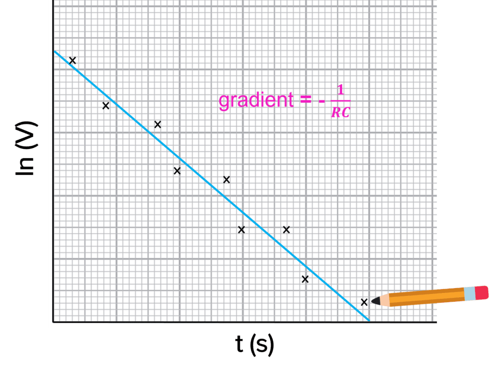
\begin{aligned} \textcolor{2730e9}{y} &= \textcolor{f21cc2}{m}\textcolor{00d865}{x} + \textcolor{d11149}{c} \\ \textcolor{2730e9}{\text{ln} \left(V\right)} &= \textcolor{f21cc2}{-\dfrac{1}{RC}} \times \textcolor{00d865}{t} + \textcolor{d11149}{\text{ln}\left(V_0\right)} \end{aligned}

So to calculate capacitance, you need to begin by plotting a graph of $\text{ln}\left(V\right)$ against $t$ as shown on the right.

$\text{ln} \left(V\right)$ must be plotted on the y-axis and $t$ must be plotted on the x-axis. This then means the gradient will be equal to $\textcolor{f21cc2}{-\dfrac{1}{RC}}$ .

So then to calculate the capacitance of the capacitor, we simply rearrange for $C$ using our calculated gradient:

$\text{gradient} = \textcolor{f21cc2}{-\dfrac{1}{RC}}$

$C = -\dfrac{1}{R \times \text{gradient}}$