
Revise
Numerical Integration
Numerical Integration
There are times when algebraic methods (integration) don’t allow you to find the area under a curve. Numerical methods can be then used for definite integrals.
Make sure you are happy with the following topics before continuing.


A Level Maths Predicted Papers 2026
Our A Level Maths Predicted Papers are produced to the same high standard as real A Level exam papers. Every question is written and reviewed by experienced exam specialists to ensure the level of challenge, structure and presentation closely reflect genuine A Level maths exams. Each pack includes professionally printed papers alongside physical mark schemes, giving students an accurate, exam-style experience that cannot be replicated with PDFs or generic revision sheets. Select your exam board and receive exclusive A Level maths predicted papers available only from MME.
View Product
A-A* A Level Maths Practice Papers
The MME A-A* A level maths practice papers are excellent for those top achieving students to practise for their exams, using authentic exam style questions that are unique to our practice papers. Our content experts have studied A level maths past papers and specifications to develop specific A-A* A level maths exam questions in an authentic exam style. The profit from every pack is reinvested into making free content on MME, which benefits millions of learners across the country.
View ProductTrapezium Rule
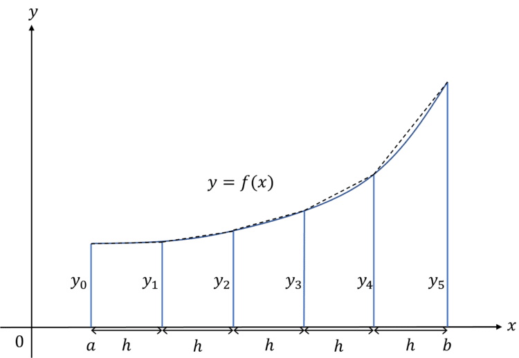
To find an approximate area under a curve we can split the area into multiple trapeziums and then add the areas of these trapeziums together.
The area of each trapezium is given by the formula:
\Large{A=\dfrac{h}{2}(y_n+y_{n+1})}
Then the area represented by \int^{b}_{a} y\,dx is approximated by:
\Large{\int^{b}_{a} y\,dx \approx \dfrac{h}{2}[y_0+2(y_1+y_2+ ... + y_{n-1})+y_n]}
- \boldsymbol{n} is the number of intervals
- \boldsymbol{h} is the width of each interval, where \boldsymbol{h=\dfrac{(b-a)}{n}}
- \boldsymbol{y_0, y_1, ... , y_n} are the heights of the sides of the trapeziums, these are obtained by substituting the appropriate x-values into the equation of the curve.
Underestimates / Overestimates
Naturally, when using approximation methods you will either get an underestimate or overestimate of the true value of the area. The shape of the curve dictates whether your approximation will an underestimate or overestimate.
If the slanted side of the trapeziums are above the curve then the approximation for the area will be an overestimate – this is the case for convex curves.
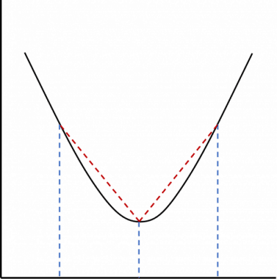
If the slanted side of the trapeziums are below the curve then the approximation for the area will be an underestimate – this is the case for concave curves.

Upper and Lower Bounds
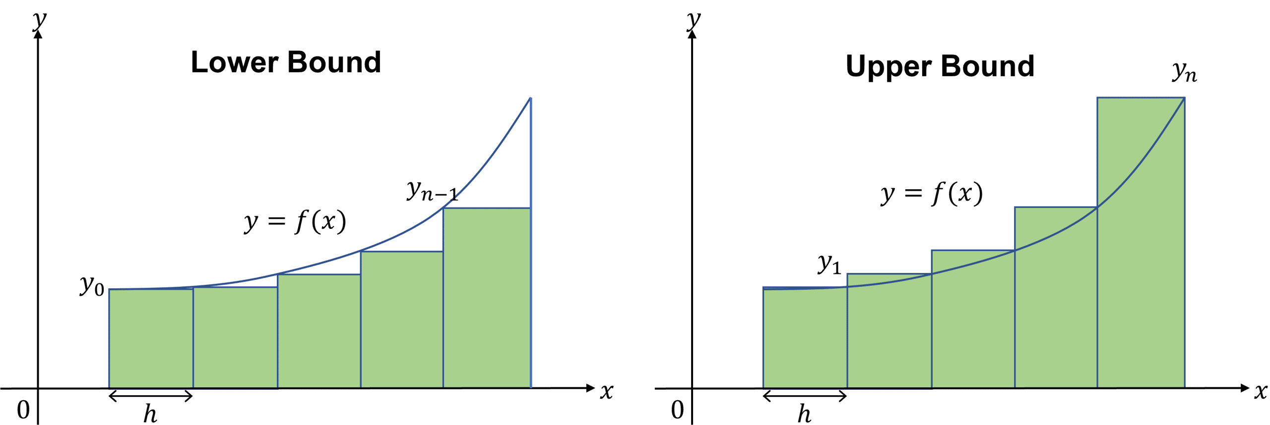
The trapezium rule will give an approximation between two bounds for the area under a curve. These upper and lower bounds are found by considering rectangular strips that lie above and below the curve respectively.
One bound is found by summing the areas of the rectangles which meet f(x) with their left hand corner, using the formula:
\int^{b}_{a}f(x) \, dx \approx h[y_0+y_1+y_2+...+y_{n-1}]
The second bound is found by summing the areas of the rectangles which meet f(x) with their right hand corner, using the formula:
\int^{b}_{a} f(x) \, dx \approx h[y_1+y_2+y_3+...+y_{n}]
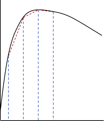
If you are calculating the bounds of a curve with a turning point you will need to use the formula for one bound on one side of the turning point and the formula for the other bound on the other side.
Integration is the Limit of the Sum of Rectangles
Using the limit of the sum of rectangles to find a definite integral uses a similar idea to differentiating from first principles.
Differentiating from first principles involves finding the gradient of a straight line between two points on a curve of an interval. As the interval, \delta x, gets smaller and smaller (\delta x \to 0), the gradient of this straight line gets closer to the gradient of the curve at these points.
We can use the area of rectangles to find the definite integral between two points:
The area of each rectangle is: \text{height} \times \text{width}=f(x)\times \delta x
So the approximate area under the curve is the sum of the areas of the rectangles, which is written as:
\Large{\sum ^{b}_{x=a+\delta x} f(x)\delta x}
Like with differentiation. the smaller the intervals the more accurate the approximation. Therefore, as \delta x \to 0 the sum of the area of the rectangles approaches the definite integral.
This can be written as:
\Large{\lim\limits_{\delta x\to0} \sum ^{b}_{a+\delta x} f(x)\delta x=\int^{b}_{a}f(x) \, dx}
Example 1: Numerical Integration
Find an approximate value for \int^{3}_{1}\sqrt{x^3+2} \, dx using 5 strips. Give your answer to 3 significant figures.
First the width of each interval needs to be calculated:
h=\dfrac{(b-a)}{n}=\dfrac{3-1}{5}=0.4Therefore the x-values are x_0=1, x_1=1.4, x_2=1.8, x_3=2.2, x_4=2.6 and x_5=3.
We can work out the corresponding y-values (heights) using the equation given:
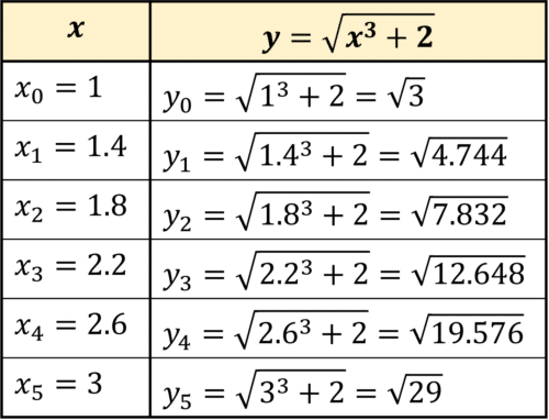
Finally, substituting the y-values into the formula: {\int^{b}_{a} y\,dx \approx \dfrac{h}{2}[y_0+2(y_1+y_2+ ... + y_{n-1})+y_n]}
\begin{aligned} \int^{3}_{1}\sqrt{x^3+2} \, dx &\approx \dfrac{0.4}{2}[\sqrt{3}+2(\sqrt{4.744}+\sqrt{7.832}+\sqrt{12.648}+\sqrt{19.576})+\sqrt{29}] \\ &=0.2[2+2\times 12.957...]\\ &=6.61 \,\, (3 \text{ sf})\end{aligned}
Example 2: Using More Intervals
Using more intervals gives you more accurate approximations:
Use the trapezium rule to approximate the area of \int^{0.5}_{0}2x\cos{2x} \, dx to 3 decimal places, with n=2 and n=4.
For n=2, the width of each strip, h=\dfrac{0.5-0}{2}=0.25.
Therefore, x_0=0, x_1=0.25 and x_2=0.5
Substituting these values into the equation gives the y-values:
y_0=0, y_1=0.4387... and y_2=0.5403...
Then using these values for the trapezium rule formula:
\begin{aligned} \int^{0.5}_{0}2x\cos{2x} \, dx & \approx \dfrac{0.25}{2}[0+2(0.5\cos{0.5})+\cos(1)] \\ &= 0.177 \end{aligned}For n=4, the width of each strip, h=\dfrac{0.5-0}{4}=0.125.
Therefore, x_0=0, x_1=0.125, x_2=0.25, x_3=0.375 and x_4=0.5
Substituting these values into the equation gives the y-values:
y_0=0, y_1=0.242..., y_2=0.4387..., y_3=0.548... and y_4=0.5403...
Then using these values for the trapezium rule formula:
\begin{aligned} \int^{0.5}_{0}2x\cos{2x} \, dx & \approx \dfrac{0.125}{2}[0 + 2(0.25\cos{0.25} + 0.5\cos{0.5}+0.75\cos{0.75}) + \cos(1)] \\ & = 0.187\end{aligned}Comparing this with the exact answer that can be found by using integration by parts, the exact value for this integral is 0.191 to 3 decimal places, so we can see that using n=4 gives us an answer which is closer to the actual area.
Numerical Integration Example Questions
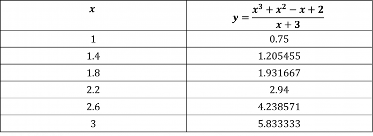
Question 1: Use the trapezium rule to estimate the value of \int^{3}_{1} \dfrac{(x^3+x^2-x+2)}{(x+3)} \, dx to 3 decimal places using 5 intervals.
[4 marks]
First we need to find the value of h:
h=\dfrac{3-1}{4}=0.4So the x-values are:
x_0=1, x_1=1.4, x_2=1.8, x_3=2.2, x_4=2.6 and x_5=3
Substituting these values into the equation gives the y-values:
Now using the trapezium rule formula:
\begin{aligned} \int^{3}_{1} \dfrac{(x^3+x^2-x+2)}{(x+3)} \, dx & \approx \dfrac{0.5}{2} [0.75+2(1.205455+1.931667+2.94+4.238571)+5.833333] \\ &= 5.443 \, (3 \text{ d.p.}) \end{aligned}

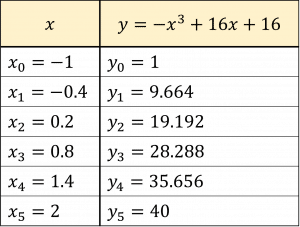
Question 2: Use the trapezium rule to estimate the value of \int^{2}_{-1} -x^3+16x+16 \, dx using 5 intervals.
Calculate \int^{2}_{-1} -x^3+16x+16 \, dx algebraically to decide whether your approximation was an underestimate or an overestimate.
[6 marks]
First we need to find the value of h:
h=\dfrac{2-(-1)}{5}=0.6So the x-values are:
x_0=-1, x_1=-0.4, x_2=0.2, x_3=0.8, x_4=1.4 and x_5=2
Substituting these values into the equation gives the y-values:
Now using the trapezium rule formula:
\begin{aligned} \int^{2}_{-1}-x^3+16x+16 \, dx &\approx \dfrac{0.6}{2}[1+2(9.664+19.192+28.288+35.656)+40] \\ &=67.98 \end{aligned}
Integrating Algebraically:
\begin{aligned} \int^{2}_{-1} -x^3+16x+16 \, dx &=[-\dfrac{x^4}{4}+8x^2+16x]^{2}_{-1} \\ &=[-\dfrac{(2)^4}{4}+8(2)^2+16(2)]-[-\dfrac{(-1)^4}{4}+8(-1)^2+16(-1)]\\&=68.25 \end{aligned}
So we can see that our approximation is an underestimate.
Question 3: Use the graph below of y=x^3-7x+1 to decide whether using the trapezium rule to estimate \int^{0}_{-2} x^3-7x+1 \, dx would be an underestimate or overestimate.
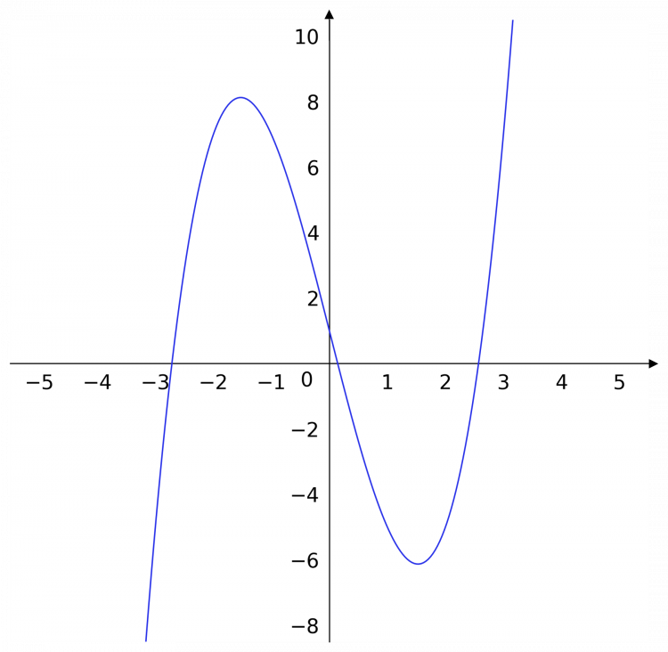
[2 marks]
Between -2 and 0, the shape of the curve is concave, therefore if the trapezium rule was used it would give an underestimate for the area under the curve.
Specification Points Covered
I3 – Understand and use numerical integration of functions, including the use of the trapezium rule and estimating the approximate area under a curve and limits that it must lie between
I4 – Use numerical methods to solve problems in context