Modelling Exponential Growth and Decay
Modelling Exponential Growth and Decay Revision
Modelling Exponential Functions and the Natural Logarithm
It is important to know how to use e^{x} and \ln(x) in real life. This means you will need to be able to sketch graphs of e^{ax+b}+c and \ln(ax+b), and interpret word-based problems about growth and decay.

Exponential Function Graphs
You need to know how to sketch y=e^{ax+b}+c. The best way to do this is step by step.
Step 1: Find where the graph intercepts the axes.
y-axis is at x=0, so y-intercept is at y=e^{b}+c
x-axis is at y=0, so x-intercept is at e^{ax+b}+c=0, which is an equation we know how to solve. Note that if c>0 the graph does not cross the x-axis.
Step 2: Find the asymptotes by looking at the behaviour of the graph as x\rightarrow\pm\infty.
As x\rightarrow\infty, y=e^{ax+b}+c\rightarrow\infty if a>0
and y=e^{ax+b}+c\rightarrow c if a<0
As x\rightarrow -\infty, y=e^{ax+b}+c\rightarrow c if a>0
and y=e^{ax+b}+c\rightarrow\infty if a<0
Step 3: Mark all of this information on a graph and use it to plot the graph.

Natural Logarithm Graphs
You need to know how to sketch y=\ln(ax+b). The best way to do this is step by step.
Step 1: Find where the graph intercepts the axes.
y-axis is at x=0, so y-intercept is at y=\ln(b)
x-axis is at y=0, so x-intercept is at ax+b=1, which is
x=\dfrac{1-b}{a}
Step 2: Find the asymptotes by looking at the behaviour of the graph as x\rightarrow\pm\infty.
If a>0, as x\rightarrow\infty, y=\ln(ax+b)\rightarrow\infty and x can decrease until ax+b=0, so there is an asymptote at x=\dfrac{-b}{a} where
y\rightarrow -\infty
If a<0, as x\rightarrow -\infty, y=\ln(ax+b)\rightarrow \infty and x can increase until ax+b=0, so there is an asymptote at x=\dfrac{-b}{a} where
y\rightarrow -\infty
Step 3: Mark all of this information on a graph and use it to plot the graph.


Modelling Exponential Growth and Decay
Most real world problems about exponential functions involve either something increasing (growth) or decreasing (decay). The maths in these problems is not new, but it is not trivial to interpret what the questions are asking.
Example: A radioactive particle decays according to R=Ae^{-0.05t}, where R is radioactivity and t is time. It starts with a radioactivity of 500.
i) Find A
ii) Find the half-life of the particle.
[6 marks]
i) At t=0, R=500
500=Ae^{-0.05\times0}
500=Ae^{0}
500=A\times1
A=500
ii) The half-life is when the radioactivity has halved, so at R=\dfrac{500}{2}=250
250=500e^{-0.05t}
\dfrac{250}{500}=e^{-0.05t}
e^{-0.05t}=\dfrac{1}{2}
-0.05t=\ln\left(\dfrac{1}{2}\right)
\begin{aligned}t&=\dfrac{-\ln\left(\dfrac{1}{2}\right)}{0.05}\\[1.2em]&=13.9\end{aligned}
A Level Maths Predicted Papers 2024
The MME A level maths predicted papers are an excellent way to practise, using authentic exam style questions that are unique to our papers. Our examiners have studied A level maths past papers to develop predicted A level maths exam questions in an authentic exam format. The profit from every pack is reinvested into making free content on MME, which benefits millions of learners across the country.

A Level Maths Revision Cards
The best A level maths revision cards for AQA, Edexcel, OCR, MEI and WJEC. MME is here to help you prepare effectively for your A Level maths exams. The profit from every pack is reinvested into making free content on MME, which benefits millions of learners across the country.


Example 1: Sketching an Exponential Graph
Sketch y=e^{3x+2}-11, marking any asymptotes and intersections with the axes.
[3 marks]

Example 2: Sketching a Logarithmic Graph
Sketch y=\ln(6x+5), marking any asymptotes and intersections with the axes.
[3 marks]

Modelling Exponential Growth and Decay Example Questions
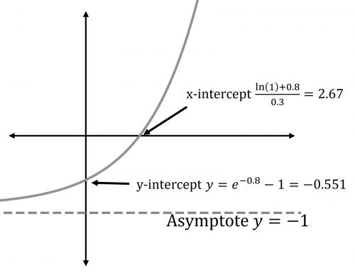
Question 1: Plot the graph y=e^{0.3x-0.8}-1, labelling where the graph crosses the axes and any asymptotes.
[3 marks]
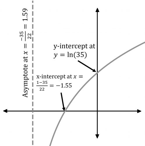
Question 2: Plot the graph y=\ln(22x+35), labelling where the graph crosses the axes and any asymptotes.
[3 marks]
Question 3: The population of a small city grows according to P=10000e^{0.1(t-2008)} where P is the population and t is the current year.
a) In which year was the city’s population first measured, and what was the population in this year?
b) What is the city’s population in 2021?
c) How many years will it take for the city’s population to reach 100000?
[7 marks]
a) From the equation, we can see that the population was first measured in 2008.
The population in 2008 was:
\begin{aligned}P&=10000e^{0.1(2008-2008)}\\[1.2em]&=10000e^{0.1\times0}\\[1.2em]&=10000e^{0}\\[1.2em]&=10000\times1\\[1.2em]&=10000\end{aligned}
b) t=2021
\begin{aligned}P&=10000e^{0.1(2021-2008)}\\[1.2em]&=10000e^{0.1\times13}\\[1.2em]&=10000e^{1.3}\\[1.2em]&=36700\end{aligned}
c) P = 100000
\begin{aligned} 100000 &=10000e^{0.1(t-2008)} \\[1.2em] \dfrac{100000}{10000}&=e^{0.1(t-2008)} \\[1.2em] 10 &=e^{0.1(t-2008)} \\[1.2em] 0.1(t-2008)&=\ln(10) \\[1.2em] t-2008 & =10\ln(10) \\[1.2em] t &=2008+10\ln(10) \\[1.2em] &=2031\end{aligned}
The city’s population will reach 100000 in 2031.
Question 4: A colony of bacteria grow very quickly according to y=Ae^{kt} where y is the population and t is time in hours. At time 0 there is only 1 bacterium. At time 10 there are 1000 bacteria.
i) Find A and t.
ii) The container in which the bacteria are in can only support 72000 of them. How long until it is at capacity?
[5 marks]
i) At t=0, y=1
Ae^{k\times0}=1
Ae^{0}=1
A\times1=1
A=1
At t=10, y=1000
e^{10k}=1000
10k=\ln(1000)
\begin{aligned}k&=\dfrac{\ln(1000)}{10}\\&=0.691\end{aligned}
ii) y=e^{0.691t}
72000=e^{0.691t}
0.691t=\ln(72000)
\begin{aligned}t&=\dfrac{\ln(72000)}{0.691}\\&=16.2\text{ hours}\end{aligned}
Modelling Exponential Growth and Decay Worksheet and Example Questions
Logarithms
A LevelYou May Also Like...

MME Learning Portal
Online exams, practice questions and revision videos for every GCSE level 9-1 topic! No fees, no trial period, just totally free access to the UK’s best GCSE maths revision platform.