
Revise
Motion Along a Straight Line
Motion Along a Straight Line
Often you are asked questions where you need to calculate distance, velocity, acceleration or time with the given information in the question. In this section we look at some of the equations that can be used in calculating them.
Displacement, Speed, Velocity and Acceleration
There are some equations we need to learn that link displacement, velocity, acceleration and time. These all apply where acceleration is constant or zero.
Average velocity is the average velocity across a whole journey and is measured in \text{ms}^{-1}, although you may see it written in different forms. You are expected to convert between units. Velocity is the displacement travelled per unit of time:
\textcolor{aa57ff}{v = \dfrac{s}{t}}
- \textcolor{aa57ff}{v} is the velocity, often in metres per second \left(\text{ms}^{-1}\right)
- \textcolor{aa57ff}{s} is the displacement, often in metres \left(\text{m}\right)
- \textcolor{aa57ff}{t} is the time in seconds \left(\text{s}\right)
Example: Usain Bolt completed in his record breaking 100 \: \text{m} sprint in 9.58\: \text{s}. Calculate his average velocity.
[1 mark]
v = \dfrac{s}{t} = \dfrac{100}{9.58} = \boldsymbol{10.4} \: \textbf{ms}^{-1}
Average acceleration is the average acceleration across a portion of a journey where the object may be accelerating. It is measured in \text{ms}^{-2} but again, could be given in different units occasionally. Acceleration is the rate of change of velocity:
\textcolor{aa57ff}{a = \dfrac{\Delta v}{\Delta t}}
- \textcolor{aa57ff}{a} is the acceleration, often in metres per second squared \left(\text{ms}^{-2}\right)
- \textcolor{aa57ff}{\Delta v} is the change in velocity, often in metres per second \left(\text{ms}^{-1}\right)
- \textcolor{aa57ff}{\Delta t} is the change in time in seconds \left(\text{s}\right)
Example: Calculate the average acceleration of a Formula 1 car which accelerates from rest to 27 \: \text{ms}^{-1} in 2.6 \: \text{s} .
[2 marks]
a = \dfrac{\Delta v}{\Delta t} = \dfrac{27 - 0}{2.6} = \boldsymbol{10.4} \: \textbf{ms}^{-2}


AQA A Level Physics Predicted Papers 2026
Our A Level Physics Predicted Papers are produced to the same high standard as real examination papers. Every question is written and reviewed by Physics subject specialists to ensure the level of challenge, format and structure closely reflect genuine A Level Physics exams. Each pack includes professionally printed exam papers and physical mark schemes, providing students with a realistic exam-style experience that goes beyond PDFs or generic revision materials. Checkout below and receive exclusive predicted papers available only from MME.
View ProductMotion Graphs
A journey of an object can be represented in a graph. The two types of graph you need to be able to interpret are distance-time graphs and velocity-time graphs.
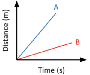
A distance-time (d-t) graph shows how the position of an object changes over time. Below are some features on a d-t graph you may see:
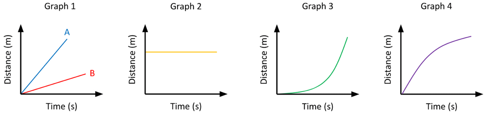
- Graph 1 shows distance increasing with time. This is the velocity of the object. The gradient represents the magnitude of the velocity. The steeper the line, the greater the velocity. So A shows a greater velocity than B.
- Graph 2 shows an object that is not changing in position over time. This represents a stationary object.
- Graph 3 shows an increase in distance with time but the curve shows that the gradient is changing. Therefore velocity is changing with time, so this represents acceleration. As the gradient increases with time, this represents a positive acceleration.
- Graph 4 also shows velocity changing over time. This one shows negative acceleration as the gradient is decreasing with time.
A velocity-time (v-t) graph shows how an object’s velocity changes over time. Some features you should recognise on a v-t graph are shown below:
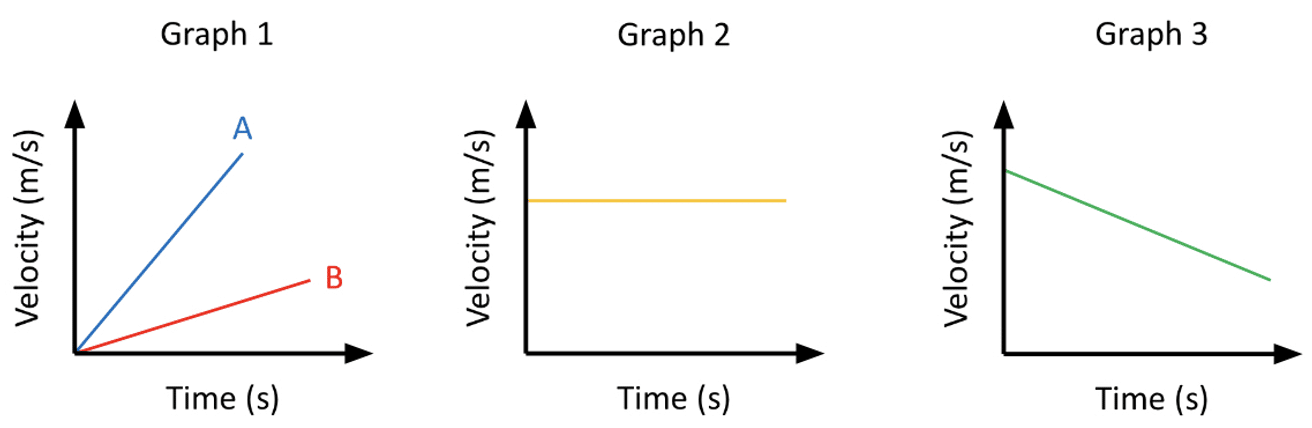
- In Graph 1, velocity is increasing over time. This shows a constant rate of acceleration. The greater the gradient, the greater the acceleration. So line A shows a greater positive acceleration than line B.
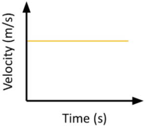
- Graph 2 shows a constant velocity over time. This represents an object moving at a constant velocity where there is no acceleration.
- Graph 3 shows velocity decreasing over time. This is a constant negative acceleration (deceleration). The more negative the gradient, the more deceleration.
Distance can also be determined from a v-t graph. As distance is equal to \text{velocity} \times \text{time} \left(d = v \times t\right) hence, the area under a velocity-time graph represents the distance.
Example: Calculate the distance travelled using the v-t graph.
[2 marks]
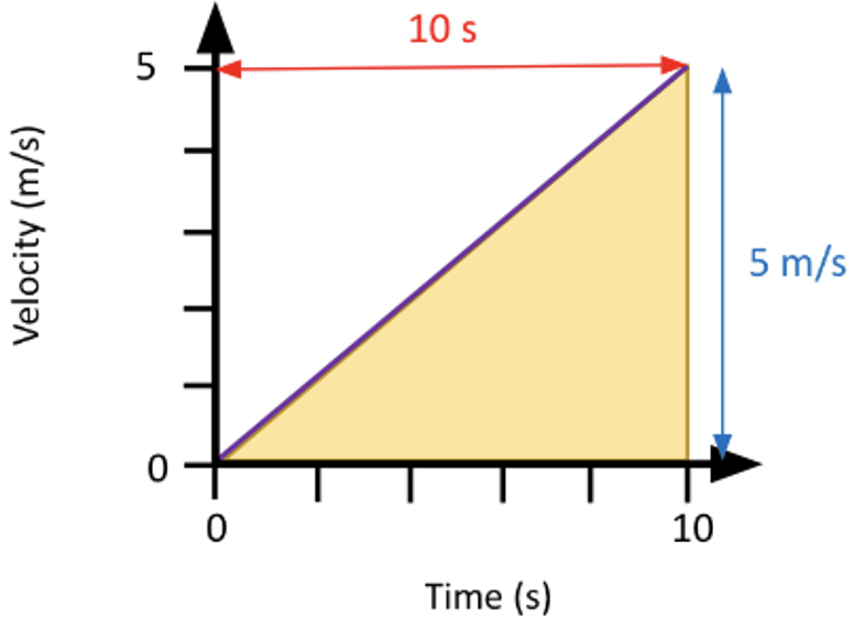
We know that the area under a velocity-time graph represents the distance. The area is a triangle, so:
d = \boldsymbol{\dfrac{1}{2} \times \left(5 \times 10\right) = 25} \: \textbf{m}
For more complex graphs you may need to break the graph down into smaller sections and calculate the area of each section before adding all the areas together.

SUVAT Equations
SUVAT equations, sometimes called the equations of motion, are named after the quantities included within the equations:
- \textcolor{00bfa8}{s = \text{Displacement} \left(\text{m}\right)}
- \textcolor{00bfa8}{v = \text{Initial Velocity} \left(\text{ms}^{-1}\right)}
- \textcolor{00bfa8}{u = \text{Final Velocity} \left(\text{ms}^{-1}\right)}
- \textcolor{00bfa8}{a = \text{Acceleration} \left(\text{ms}^{-2}\right)}
- \textcolor{00bfa8}{t = \text{Time} \left(\text{s}\right) }
SUVAT equations can be used to work out different quantities for moving objects. As long as you have 3 of the values above, you will be able to work out whichever other quantity you want to know.
The SUVAT equations are given on your data sheet and include:
\textcolor{00bfa8}{v = u + at}
\textcolor{00bfa8}{ s = ut + \dfrac{1}{2} a t^2}
\textcolor{00bfa8}{s = \dfrac{\left(v+u\right) t}{2}}
\textcolor{00bfa8}{v^2 = u^2 + 2as}
As each of the equations contain different combinations of our quantities, you may decide which equation to use by picking the one that includes the information given to you in a question and the quantity you are looking for. Some questions may involve multiple steps in which you use more than one of the SUVAT equations.
Example: A cyclist starts to cycle from rest. They accelerate at a constant acceleration of 2.5 \: \text{ms}^{-2} for 15 seconds. Pick a SUVAT equation and calculate the cyclists velocity after 15 seconds.
[3 marks]
S= \: ? (We don’t need this for this question)
U= 0 \: \text{ms}^{-1} (any object from rest has u = 0)
V= \: ? (This is the unknown we wish to find)
A= 2.5 \: \text{ms}^{-2}
T= 15 \: \text{s}
So we know u, a, and t. We want to find v, so we use the following SUVAT equation:
\boldsymbol{v = u + at}
v = \boldsymbol{0+ \left(2.5 \times 15 \right) }
v = \boldsymbol{37.5} \: \textbf{ms}^{-1} \boldsymbol{=} \boldsymbol{38} \: \textbf{ms}^{-1} \left( 2 \: \text{sf} \right)
Required Practical 3
Determination of g by a freefall method.
This experiment will involve dropping an object and measuring the time taken for it to fall. The aim is to calculate a relatively accurate value for the acceleration due to gravity on earth, g. This experiment can be done with many different objects and different set ups, however a simple and effective method is the one we will detail here.
Doing the Experiment:
- Set up the experiment as shown in the diagram.
- The light gates and data logger should be set up to record the time taken to for the ball to pass between the light gates.
- Attach the ball to the electromagnet at the top of the equipment setup. The electromagnet should remain on until the experiment is ready to start.
- Measure the distance between the light gates. This is h, and an appropriate starting value for h would be 10 \: \text{cm}.
- Close the switch in the electromagnet circuit so that the electromagnet switches off and the ball is released.
- Record the time taken \left(\textcolor{10a6f3}{t}\right) for the ball to travel between the light gates from the datalogger.
- Repeat the process with different heights, varying the height h by 5 \: \text{cm} each time.
- Each height should be repeated a minimum of 5 times and a mean of the time taken for each height should be calculated.
Analysing the results:
Once the results have been collated and we have our heights and their corresponding average times, we can begin to calculate g. First we need to look at the following SUVAT equation and rearrange it:
\begin{aligned} s &= ut + \dfrac{1}{2} a t^2 \\ \dfrac{2s}{t} &= at + 2u \end{aligned}
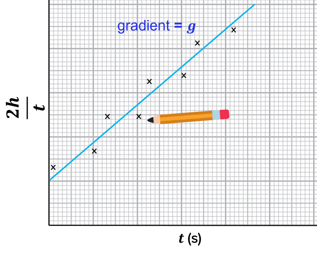
We can replace s with our height from the experiment, h, and replace the acceleration a with the gravitational acceleration, g. We can then compare this to the straight line equation.
\begin{aligned} \textcolor{7cb447}{\dfrac{2h}{t}} &= \textcolor{2730e9}{g}\textcolor{d11149}{t} + \textcolor{aa57ff}{2u} \\ \textcolor{7cb447}{y} &= \textcolor{2730e9}{m} \textcolor{d11149}{x} + \textcolor{aa57ff}{c}\end{aligned}
Therefore, to find \textcolor{2730e9}{g} we can plot a graph of \textcolor{7cb447}{\dfrac{2h}{t}} against \textcolor{d11149}{t}. The gradient of this graph will be equal to our value of \textcolor{2730e9}{g}.
There may be a few errors from this experimental procedure:
- Measuring the height using a ruler can cause a random error because a large uncertainty can arise from the ruler due to it’s resolution of 1 \: \text{mm}.
- Parallax error can arise from the student recording the value of h.
There are more possible errors that could arise, but repeating the experiment and calculating mean values will ensure that these errors have little effect on the experiment.
Motion Along a Straight Line Example Questions
Question 1: A passenger plane takes 20 seconds to reach a velocity fast enough to take-off. The minimum take-off velocity is 82 \: \text{ms}^{-1}. Calculate the average acceleration of the plane and explain this is an average acceleration.
[3 marks]
\begin{aligned} a &= \dfrac{\Delta v}{\Delta t} \\ \\ a &= \dfrac{\left(82-0\right)}{20} = 4.1 \: \text{ms}^{-2} \end{aligned}
This is an average acceleration because the acceleration may vary over the \boldsymbol{20} seconds.

Question 2: Describe how you would recognise a constant velocity from a distance-time graph and a velocity-time graph.
[2 marks]
In a distance-time graph, a constant velocity is given by the gradient of a line with increasing velocity over time:
In a velocity time graph a constant velocity is given by a horizontal line on the graph:
Question 3: A ball is dropped from a height of 5 \: \text{m} . Calculate velocity of the ball the instant it hits the ground.
[3 marks]
- s = 5 \: \text{m}
- u = 0 \: \text{ms}^{-1}
- v \: = ? (This is the unknown we wish to find)
- a = 9.81 \: \text{ms}^{-2} (This is the value for any object in free fall)
- t \: = ? (We don’t need this for this question)
Because u = 0 \: \text{ms}^{-1} we can write this as:
\begin{aligned} v^2 &= 2as \\ \boldsymbol{v^2} &\boldsymbol{= 2 \times 9.81 \times 5} \\ v &= \sqrt{98.1} = \boldsymbol{9.9} \: \textbf{ms}^{-1} \end{aligned}
Specification Points Covered
AQA A Level:
- 3.4.1.3 Motion along a straight line