
Revise
Limitations and Errors in Measurements
Limitations and Errors in Measurements
All measurements we take will have limitations and a certain degree of error. It is important to understand how to describe and categorise errors, identify limitations of measurements, and calculate uncertainties.
Types of Errors
However much we try to control an experiment, we cannot entirely prevent errors. We can work to minimise the effects of these errors as much as possible if we can identify them. Errors can fall into different categories:
Random Errors
Random errors are very common in most experiments. A random error causes variations in results in both directions (too high or too low) and are usually uncontrollable. For example, environmental conditions may be a source of random error. Because they are mostly uncontrollable, we can find ways to reduce their impact. The best way to reduce the effect of random errors in an experiment is to take multiple readings, remove anomalies and take an average of your readings. The more repeat readings you take, the more the impact of the random error is reduced. Usually we would suggest taking a minimum of 5 repeat readings.
Systematic Errors
Systematic errors are more easily controlled and prevented as these arise from faulty equipment or poor experimental design. They always act in one direction. For example, if we used a vernier calliper that had been damaged so that its readings were always 1mm too large, we could account for this in our results. The error is repeated each time so can easily be accounted for or removed by using another piece of equipment. Systematic errors can be removed by planning carefully and calibrating equipment before use.
Zero Errors
A zero error is a specific type of systematic error, usually caused by not calibrating equipment correctly. This occurs when a piece of measuring equipment has a positive or negative reading before being used. The measurement will always be incorrect by this amount every time. If no alternative equipment is available, then this can be taken into account before processing results.


AQA A Level Physics Predicted Papers 2026
Our A Level Physics Predicted Papers are produced to the same high standard as real examination papers. Every question is written and reviewed by Physics subject specialists to ensure the level of challenge, format and structure closely reflect genuine A Level Physics exams. Each pack includes professionally printed exam papers and physical mark schemes, providing students with a realistic exam-style experience that goes beyond PDFs or generic revision materials. Checkout below and receive exclusive predicted papers available only from MME.
View ProductPrecision and Accuracy
Precision
If measurements are to be precise, they are all very close to the mean average value. This does not necessarily mean they are accurate, but it means that the results are all very close together.
One way of making results more precise is by using another piece of equipment that records to a higher number of decimal places.
Accuracy
If results are accurate, they are close to the true value. The closer a measurement is to the true value, the more accurate the reading. Ideally, a set of results would be both accurate and precise.
Repeatability and Reproducibility
Repeatability
If the same person can repeat the same method with the same equipment, then the results show high repeatability. For repeatability it has to be the same person and equipment.
Reproducibility
If a different person can obtain the same results, or the same results can be measured using different equipment or methods, then the results are reproducible.
Resolution
Resolution is the smallest measurable change that can be made using an instrument. For example, the resolution of a stopwatch is usually 0.01 \: \text{s}. It is the smallest increment of change that the measuring instrument can detect.
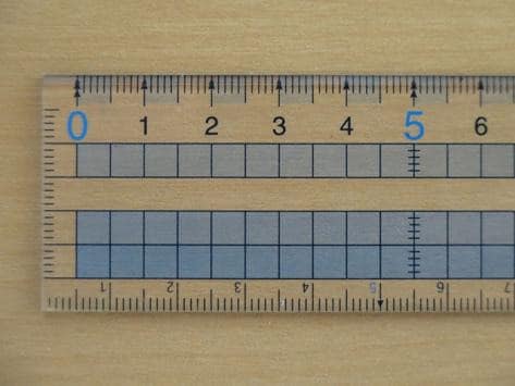
The smallest increment on the ruler is 1 \: \text{mm}. Therefore its resolution is 1 \: \text{mm} .
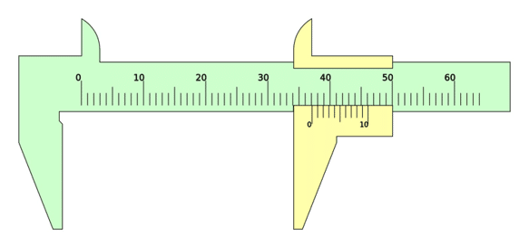
The smallest increment on the vernier calliper is 0.1 \: \text{mm}. Therefore its resolution is 0.1 \: \text{mm}.
Representing and Calculating Uncertainties
The uncertainty of a measurement is the range in which the true reading should be expected to lie. Any measurement has a degree of uncertainty based on the resolution of the measuring instrument. Usually, the better the resolution of the equipment, the smaller the uncertainty. Uncertainties can be represented in three ways:
- Absolute uncertainty: The uncertainty is given as a fixed value above and below the true reading e.g. 20 ± 1 \: \text{cm}.
- Fractional uncertainty: The uncertainty is given as a fraction of the true value e.g. 20 ± 1/20 \: \text{cm}.
- Percentage uncertainty: The uncertainty is given as a percentage of the true value e.g. 20 ± 0.5 \% \: \text{cm}.
If we take a set of measurements from an experiment, each measurement will have its own uncertainty. If we then use these measurements in a calculation, we need to be able to calculate the uncertainty in the new value we have calculated. This is where we need to combine uncertainties.
Adding and Subtracting using Uncertainties
- If we add or subtract two measurements, we need to add the absolute uncertainties of each measurement together:
If we were calculating the temperature change of a piece of metal being heated from initial temperature 293±0.5 \: \text{K} and final temperature 315±0.5 \: \text{K}, then the temperature change would be represented as 22±\: \text{1} K (the uncertainties are added together).
It’s important to note that this method only works with absolute uncertainties and would not apply with fractional or percentage uncertainties.
Multiplying and Dividing using Uncertainties
- If we are multiplying or dividing two measurements, the percentage uncertainties should be added. Again, this will not work for absolute or fractional uncertainties.
Let’s say we needed to calculate the resistance of a wire having measured the current and voltage. If the current is measured to be 1.0±0.1 \text{A} and the voltage 6±0.5\: \text{V}, we could use the equation R =\dfrac{V}{I} to calculate the resistance and add the percentage uncertainties.
But first, the percentage uncertainties need to be calculated:
Current: \dfrac{0.1}{1} = 0.1 \%, Voltage: \dfrac{0.5}{6.0}= 0.083 \%
Then we add the percentage uncertainties together to give the uncertainty of the resistance:
0.1 \% + 0.083 \% = 0.183 \%Therefore, the percentage uncertainty of the resistance is: 6± 01.83 \% Ohms.
Uncertainties and Powers
- Finally, if we are raising a measurement to a power, then the percentage uncertainties are multiplied by the power.
If we have a cube of which we wish to measure the volume and know that one length of the cube is 5± 0.1 \: \text{cm}, then again, we first must calculate the percentage uncertainties.
\dfrac{0.1}{5}= 0.02 \%.
Now we can multiply the percentage uncertainty by 3 as the volume of the cube is the length of the side raised to the power of 3.
Volume = 5 \times 5 \times 5 = 125 \: \text{cm} and the uncertainty is 0.02 \times 3 = 0.06 \%.
Therefore the volume is represented as 125 \: \text{cm}^3 ±0.06 \%
Example: Describing accuracy and Precision
Four students are using different equipment and methods to measure the diameter of a wire. We are told the true diameter of the wire is 5 \: \text{mm}.
Below are the results of the investigation. Which student do you think has recorded the most accurate and precise results?
| Student 1 | Student 2 | Student 3 | Student 4 |
| 5.00 | 6.0 | 6.00 | 6.0 |
| 5.20 | 4.0 | 6.10 | 7.0 |
| 4.90 | 5.0 | 5.90 | 5.0 |
| 4.80 | 4.5 | 5.80 | 6.5 |
| 5.10 | 5.5 | 6.10 | 5.5 |
| Average: 5.00 | Average: 5.0 | Average: 6.00 | Average: 6.0 |
[4 marks]
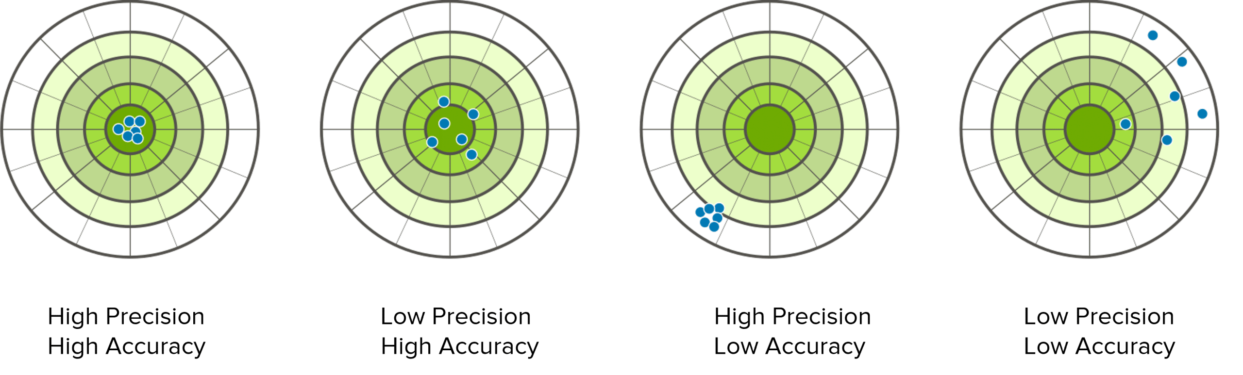
Student 1: This set of results are the most accurate AND precise. They are close to the true value and all the results are close to the mean value. This is the best set of results out of the 4 students.
Student 2: this set of results are also the most accurate, but not the most precise. They get an average that is close to the true value, but the results are spread out more than student 1 so they are not precise.
Student 3: this set of results are also the most precise but not the most accurate. They are all close together showing precision, but the mean is not close to the true value. We could note that this may be due to a zero error of 1mm.
Student 4: Finally, this set of results are the least accurate and least precise. They do not come close to the true mean and the results are spread out.
Therefore, Student 1 has used a method and set of equipment that produces the most accurate and precise results.
This can also be represented visually:
Limitations and Errors in Measurements Example Questions
Question 1: A student is calculating the specific heat capacity of a variety of metal blocks.
To calculate this, they must know the mass of the metal blocks. They use a top pan balance to measure the masses but forget to zero the balance and the reading shows 1.5 \: \text{g} before anything is put on the scales.
What type of error is this and how should the student deal with it?
[3 marks]
This is a systematic (zero) error. It means all the measurements will be too high by 1.5 \: \text{g}. To eliminate this type of error, all the masses should be reduced by \boldsymbol{1.5} \: \textbf{g} before any calculations are made.

Question 2: A student stated that their calculated value for acceleration due to free fall is 9.5±0.5 \: \text{ms}^{-2}. What does this tell you about their value for acceleration?
[2 marks]
This tells us that there is a degree of uncertainty due to the measurements they have used. The true value for acceleration is somewhere between \boldsymbol{9 \: \textbf{ms}^{-2} } and \boldsymbol{10 \: \textbf{ms}^-2}.
Question 3: Calculate the percentage uncertainty of the acceleration calculated using the equation F=ma where F= 900.0±1.0 \: \text{ N} and m= 72.0±0.1 \: \text{ kg}.
[3 marks]
Firstly, calculate the percentage uncertainties.
\boldsymbol{\dfrac{1}{900}= 0.001 \%} for Force, and \boldsymbol{\dfrac{0.1}{72}= 0.0138} \% for mass.
Now calculate the acceleration and add the uncertainties:
\begin{aligned} \\ a &=\dfrac{F}{m} \\ \\ a&= \dfrac{900}{72} = 12.5\: \text{ms}^{-2} \end{aligned}
So the acceleration = \boldsymbol{12.50 \:} \textbf{ms}^{-2} \boldsymbol{±0.01 \%} .
Specification Points Covered
AQA A level:
- 3.1.2 Limitation of physical measurements