
Revise
Reduction to Linear Form
Reduction to Linear Form
Some exponential equations can be reduced to a form that looks like y=mx+c. Specifically, after applying the laws of logarithms we can treat y=ax^{n} and y=ab^{x} as if they were linear equations.


A Level Maths Predicted Papers 2026
Our A Level Maths Predicted Papers are produced to the same high standard as real A Level exam papers. Every question is written and reviewed by experienced exam specialists to ensure the level of challenge, structure and presentation closely reflect genuine A Level maths exams. Each pack includes professionally printed papers alongside physical mark schemes, giving students an accurate, exam-style experience that cannot be replicated with PDFs or generic revision sheets. Select your exam board and receive exclusive A Level maths predicted papers available only from MME.
View Product
A-A* A Level Maths Practice Papers
The MME A-A* A level maths practice papers are excellent for those top achieving students to practise for their exams, using authentic exam style questions that are unique to our practice papers. Our content experts have studied A level maths past papers and specifications to develop specific A-A* A level maths exam questions in an authentic exam style. The profit from every pack is reinvested into making free content on MME, which benefits millions of learners across the country.
View Product\mathbf{y=ax^{n}}
y=ax^{n}Take logarithms:
\begin{aligned}\log(y)&=\log(ax^{n})\\[1.2em]&=\log(a)+\log(x^{n})\\[1.2em]&=\log(a)+n\log(x)\end{aligned}
Overall we have:
y=ax^{n}\Rightarrow \log(y)=\log(a)+n\log(x)
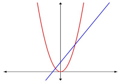
Now if we plot \log(y) against \log(x), we have a straight line graph.
The graph below shows y against x in red and \log(y) against \log(x) in blue. As expected, the blue line is straight.
\mathbf{y=ab^{x}}
y=ab^{x}Take logarithms:
\begin{aligned}\log(y)&=\log(ab^{x})\\[1.2em]&=\log(a)+\log(b^{x})\\[1.2em]&=\log(a)+x\log(b)\end{aligned}
Overall we have:
y=ab^{x}\Rightarrow \log(y)=\log(a)+x\log(b)
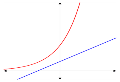
Now if we plot \log(y) against x, we have a straight line graph.
The graph below shows y against x in red and \log(y) against x in blue. As expected, the blue line is straight.
Example 1: Converting to Linear Form
Convert y=99\times0.5^{x} to linear form.
[2 marks]
y=99\times0.5^{x}
\begin{aligned}\log(y)&=\log(99\times0.5^{x})\\[1.2em]&=\log(99)+log(0.5^{x})\\[1.2em]&=\log(99)+x\log(0.5)\end{aligned}

Example 2: Using Linear Form
The data below is taken from a plot of the form y=ax^{n}. By plotting \log_{10}(y) against \log_{10}(x), find a and n.
[5 marks]
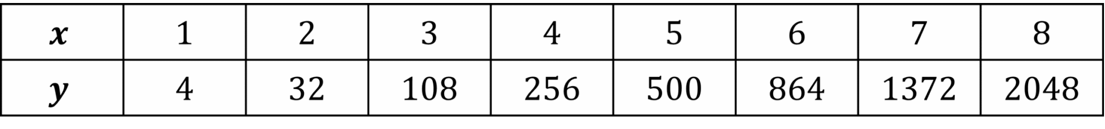
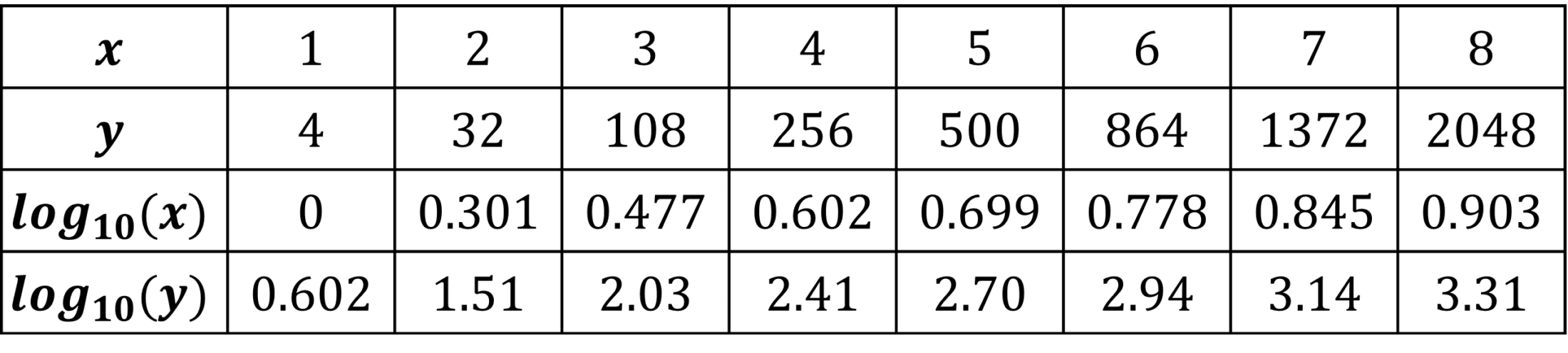
Step 1: Calculate \log_{10}(x) and \log_{10}y and put them in a table.
Step 2: Plot \log(y) against \log(x) on a scatter graph.
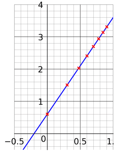
Step 3: Use the scatter graph to find the gradient and y-intercept.
Gradient is approximately \dfrac{3.3-0.6}{0.9-0}=\dfrac{2.7}{0.9}=3
y-intercept is approximately 0.6
Step 4: Use our linear form to interpret the gradient and y-intercept.
y=ax^{n}\rightarrow \log(y)=\log(a)+n\log(x)Gradient is n so n=3
y-intercept is \log(a) so \log(a)=0.6 so a=10^{0.6}=4 to two significant figures.
Step 5: Put together to determine the form of the plot:
y=4x^{3}
Reduction to Linear Form Example Questions
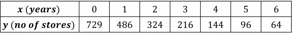
Question 1: The number of branches of a high-street store decreases over time. This trend, which is of the form y=ab^{x} is monitored over a number of years. Use the data from the monitoring to find a and b.
[5 marks]
If the question does not specify a base for logarithms it is up to us to choose a sensible base. The choice of base should not affect the answer at the end. In the working below, we have used a base of 2.
Note the linear form:
y=ab^{x}\rightarrow log(y)=x\log(b)+\log(a)So the straight line is obtained by plotting \log(y) against x.
This means that we need to add a \log(y) row to the table.
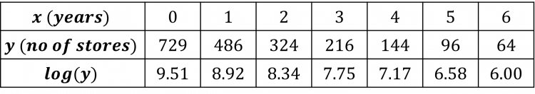
Plot \log(y) against x and add a line of best fit.
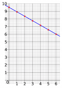
Find the gradient and the y-intercept.
Gradient is \dfrac{6-9.5}{6-0}=\dfrac{3.5}{6}=-\dfrac{7}{12}
y-intercept is 9.5
Interpret the gradient and y-intercept.
Gradient is \log(b)
\log(b)=-\dfrac{7}{12}
b=0.667
y-intercept is \log(a)
\log(a)=9.5
a=729
Put it all together:
Our estimate for the line is y=729\times0.667^{x}

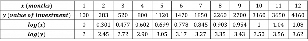
Question 2: The value of an investment in MathCoin is believed to reliably climb following an ax^{n} trajectory. Claire buys one MathCoin and monitors the price of her investment every month over one year. Find a and n.

[5 marks]
If the question does not specify a base for logarithms it is up to us to choose a sensible base. The choice of base should not affect the answer at the end. In the working below, we have used a base of 10.
Note the linear form:
y=ax^{n}\rightarrow log(y)=n\log(x)+\log(a)So the straight line is obtained by plotting \log(y) against \log(x).
This means that we need to add a \log(x) row and a \log(y) row to the table.
Plot \log(y) against \log(x) and add a line of best fit.
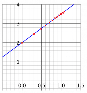
Find the gradient and the y-intercept.
Gradient is \dfrac{3.5-2}{1-0}=\dfrac{1.5}{1}=1.5
y-intercept is 2
Interpret the gradient and y-intercept.
Gradient is n
n=1.5
y-intercept is \log(a)
log(a)=2
a=100
Put it all together:
Our estimate for the line is y=100\times x^{1.5}
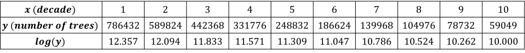
Question 3: A forest has been declining in population since the nineteenth century. To assess this decline, a census of the tree population of the forest was conducted every ten years in the twentieth century. It is believed this decline follows a y=ab^{x} curve. Use the table of census data to find a and b.

[5 marks]
Again we can choose our own base for logarithms, so we will take the logarithm with base 3.
y=ab^{x}
\begin{aligned}\log(y)&=\log(ab^{x})\\[1.2em]&=\log(a)+\log(b^{x})\\[1.2em]&=\log(a)+x\log(b)\end{aligned}
So we plot \log(y) against x, and the gradient will be \log(b) and the y intercept will be \log(a).
Plotting \log(y) against x gives this graph.
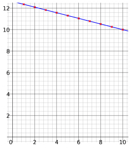
The graph goes through the points (1,12.357) and (10,10).
\begin{aligned}\text{gradient}&=\dfrac{10-12.357}{10-1}\\[1.2em]&=\dfrac{-2.357}{9}\\[1.2em]&=-0.262\end{aligned}
\log(b)=-0.262
b=3^{-0.262}
b=0.750
The graph passes through (1,12.357) and has a gradient of -0.262, so it also passes through (0,12.357+0.262)=(0,12.619)
So y intercept is 12.619
\log(a)=12.619
a=3^{12.619}
a=1048576
Hence, y=1048576\times0.750^{x}
Specification Points Covered
F6 – Use logarithmic graphs to estimate parameters in relationships of the form y=ax^n and y=kb^x, given data for x and y